In this blog post, we will learn from Zillow's incident and understand how ML monitoring tools can help you detect the early effects of model performance decay and data drift.

In November 2021, the American real-state company Zillow reported a loss of almost $500 M. Because of a failure in their machine learning model in charge of estimating house prices.

Many factors played a role in Zillow's significant loss. Some related to business decisions, but others to the lack of monitoring of their machine learning model, some speculate. Zillow never released any information about what had caused the incident.

The incident#

In 2018 Zillow funded a new branch of their business called Zillow Offers, where they buy houses from their consumers and then resell them at a higher price. Before the collapse, the new Zillow Offers branch was operating well. In fact, it was the company’s primary revenue stream.

Zillow’s price model was known for overestimating the price of houses. We don’t know exactly why they wanted a model to behave like that. But in a “hot market”, it made sense to pay the owners a little bit more to close deals faster, make minimal decorations, and sell the houses quickly at a higher price.

But, when the COVID-19 pandemic hit the world and the housing market cooled down, the company found itself with many houses to sell and no one to buy them. As a result, the company lost about $500 M, closed the Zillow Offers branch, and laid off 25% of its workforce.

Could Zillow have detected the incident in time?#

Before and during the pandemic, Zillow’s model continued to operate unchanged. Overestimating house prices as if they were on a “hot market”. The problem was that, in reality, the market was getting colder and colder.

In machine learning, this is known as concept drift. And it is one of the main reasons for model performance decay. Concept drift happens when the decision boundary patterns of the training and current data are different. This usually occurs when people’s behaviors change — as in the COVID-19 pandemic, the market conditions changed and the model did not take changes into account.

Before Zillow realized the issue, it was too late. Monitoring ML software like NannyML could have helped to detect early warnings of data drift or model performance decay and alert the company on time.

Zillow’s case was a particular event where a model probably trained with hot market assumptions was a victim of the COVID-19 pandemic — a global event that affected people’s behaviors.

What Causes Post-Deployment Model Failure?#

In general, we don’t need a global pandemic to mess up our machine-learning models. Much simpler events can cause us nightmares when speaking about post-deployment model performance. It’s known that when not monitored correctly, machine learning models can lose about 20% of their value in the first six months after being deployed.

Events like expanding the service to new cities/countries can significantly change the distribution of the new model’s inputs compared to the one used to train it.

Let’s learn how to use NannyML to spot early warnings of model performance decay and data drift.

How to Detect Model Failures Using NannyML#

Given that we don’t have access to Zillow’s official data and model, we’ll use the California House Pricing dataset in the following sections to emulate Zillow’s use case. We’ll train a machine learning model with it and build a toy example to see if we can catch any model failures.

Dependencies#

import nannyml as nml
import pandas as pd
import numpy as np
import datetime as dt

from sklearn.datasets import fetch_california_housing
from sklearn.linear_model import LinearRegression
from sklearn.ensemble import RandomForestRegressor
from sklearn.metrics import mean_absolute_percentage_error

# fetch california housing dataset using sklearn
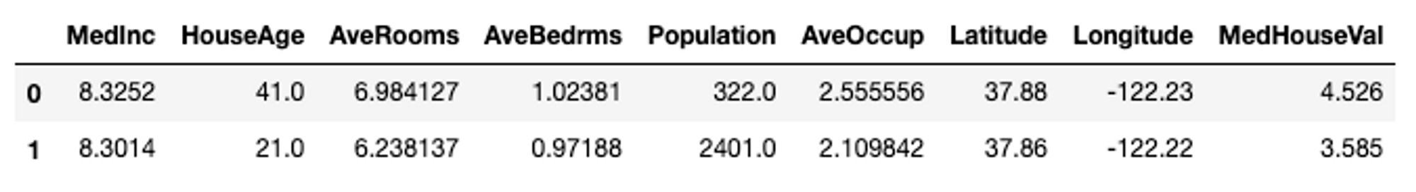
cali = fetch_california_housing(as_frame=True)
df = pd.concat([cali.data, cali.target], axis=1)
df.head(2)

Enriching the data#

Remember that NannyML does its magic with post-deployment machine learning models. Because of this, we are going to add a time dimension to our samples and split the dataset into reference and analysis sets.

We do this to simulate that data examples with older timestamps were used to train and test the model, and newer ones were run through the model at post-deployment time.

# add artificial timestamp
timestamps = [dt.datetime(2020,1,1) + dt.timedelta(hours=x/2) for x in df.index]
df['timestamp'] = timestamps

# add periods/partitions
train_beg = dt.datetime(2020,1,1)
train_end = dt.datetime(2020,5,1)
test_beg = dt.datetime(2020,5,1)
test_end = dt.datetime(2020,9,1)
df.loc[df['timestamp'].between(train_beg, train_end, inclusive='left'), 'partition'] = 'train'
df.loc[df['timestamp'].between(test_beg, test_end, inclusive='left'), 'partition'] = 'test'
df['partition'] = df['partition'].fillna('production')

Training a Machine Learning Model#

For this task, we are going to simulate Zillow’s house pricing prediction model by using a random forest regressor to estimate the MedHouseVal using HouseAge, Rooms, Bedrooms, etc., as features.

Meeting NannyML Data Requirements#

NannyML requires two datasets:

• Reference set: This is your validation set. A dataset that the model did not see during training, but we know the correct labels.
• Analysis set: This can be all the data examples that came or will come after the model has been deployed. We don’t know the real labels but can know the model’s estimation.

df_for_nanny = df[df['partition']!='train'].reset_index(drop=True)
df_for_nanny['partition'] = df_for_nanny['partition'].map({'test':'reference', 'production':'analysis'})
df_for_nanny['identifier'] = df_for_nanny.index

reference = df_for_nanny[df_for_nanny['partition']=='reference'].copy()
analysis = df_for_nanny[df_for_nanny['partition']=='analysis'].copy()
analysis_target = analysis[['identifier', 'MedHouseVal']].copy()
analysis = analysis.drop('MedHouseVal', axis=1)

# dropping partition column that is now removed from requirements.
reference.drop('partition', axis=1, inplace=True)
analysis.drop('partition', axis=1, inplace=True)

Estimating Post-Deployment Model Performance#

Now that we have the reference and analysis datasets, we can use NannyML’s magic. To do this, we will use the DLE method, short for Direct Loss Estimation.

The DLE estimates the loss resulting from the difference between the prediction and the target before the targets become known. The loss is defined from the regression specified performance metric. We will use Mean Absolute Percentage Error (MAPE) in this case.

To know more about how DLE estimates performance, read how Direct Loss Estimation works.

estimator = nml.DLE(
    feature_column_names=features,
    y_pred='y_pred',
    y_true='MedHouseVal',
    timestamp_column_name='timestamp',
    metrics=['mape'],
    tune_hyperparameters=False
)
estimator.fit(reference)
results = estimator.estimate(analysis)

After fitting the DLE estimator on the reference data and running the new estimates on the analysis set, we can plot the estimated model performance through time.

for metric in estimator.metrics:
    metric_fig = results.plot(kind='performance', metric=metric, plot_reference=True)
    metric_fig.show()

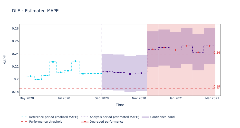
From the plot above, we can see that the Mean Absolute Percentage Error (MAPE) started to increase at post-deployment time. It seems that the model was initially making good predictions, but around November 2020, something happened, and we got a drop in performance.

Let’s see if we can figure out what changed in the data that made our model underperform after being in production for a couple of months.

Detecting Data Drift#

Data drift happens when the production data comes from a different distribution than the model’s training data.

The data drift detection functionality of NannyML can help us understand which features are drifting and the underlying problem for the drop in performance. So that we can take the proper corrective action: retrain, refactor, revert to a previous model, take the model offline, change the business process, etc.

In the NannyML workflow, we don’t use data drift detection as an alarming system but as a way to find the root cause of the issue.

The reason why is that not all features affect the model in the same way. Some are more important than others. We could find a feature drifting, but this doesn’t necessarily translate into a performance drop.

If we built a system that alerts every time it detects data drift, we would end up with many false alarms. Given that we live in a world that is constantly changing, it is normal for distributions to change. So, it’s better to monitor the model performance instead and only alert if we detect decay on it. And then use data drift detection to find the root cause of the problem.

Univariate Data Drift#

Univariate data drift checks the distribution of every variable separately to see if there has been any drift between the reference and analysis periods.

To search for univariate data drift, we are going to use the UnivariateDriftCalculator method. It allows us to apply different statistical methods, such as the Kolmogorov–Smirnov test, to compare distributions and help us detect any presence of data drift.

# create an instance of UnivariateDriftCalculator
calc = nml.UnivariateDriftCalculator(
    column_names=['HouseAge', 'AveBedrms', 'AveOccup'],
    timestamp_column_name='timestamp',
    continuous_methods=['kolmogorov_smirnov'],
)

# fit the UnivariateDriftCalculator instance on the reference data
calc.fit(reference)
# evaluate the fitted calculator on the analysis data
results = calc.calculate(analysis)

Next, let’s visualize the results. Since we are dealing with continuous variables, NannyML can plot the estimated probability distribution of the variable for each chunk in a plot called joyplot. The chunks where the drift was detected are highlighted.

for column_name in results.continuous_column_names:
    figure = results.plot(
        kind='distribution',
        column_name=column_name,
        method='kolmogorov_smirnov',
        plot_reference=True
    )
    figure.show()

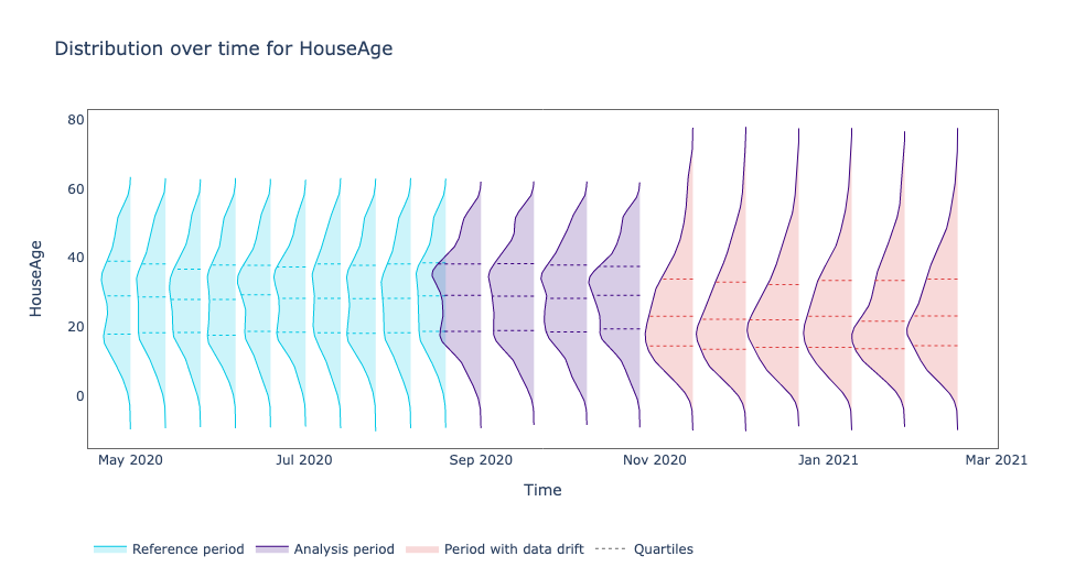
Looking at the above plot we see that there was a drift at the HouseAge feature starting from November 2020 which is also the month where we saw a performance drop from our model.

The new distribution has its mean value lower than the reference and analysis periods. Meaning, the production data contains newer houses.

This could have happened because there are new areas added to the application where houses are newer. Or maybe after covid people considered selling their houses to move to other cities and be closer to their families.

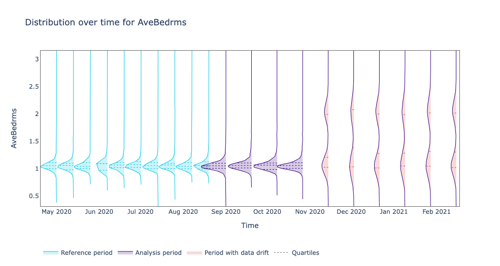
We observe an interesting phenomenon with AveBedrms. New houses seem to be bigger. Before November houses seem by the system typically had on average one bedroom but now we see a bimodal distribution of houses with one and two bedrooms.

This makes us think that maybe young families with houses of two bedrooms are now adding their house to the application and thinking about the idea of relocating to other cities. Or maybe the service is now active in new areas like a countryside where houses are typically bigger.

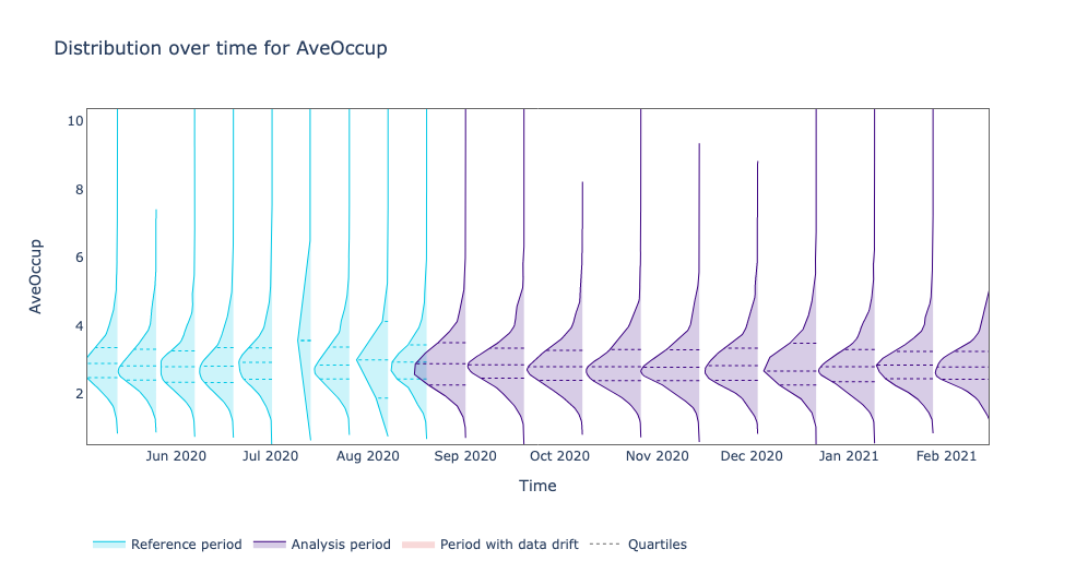
On the other hand, the AveOccup feature did not suffer any data drift. This allows us to narrow our investigation to HouseAge and AveBedrms.

Now that we know which features are causing the performance decay we can start thinking about how to fix the issue: retraining the model with newly acquire data, going back to a previous model, taking the model offline, changing the business process, etc.

But what happens when we know that there is a performance drop but we can not find any data drift in the features?

Multivariate Data Drift#

NannyML provides us with a way to detect more subtle changes in the data that cannot be detected with univariate approaches.

One method to detect such changes is Data Reconstruction with PCA. This method reduces the dimensionality of the model input data. Capturing 65% of the dataset’s variance. (This is a parameter that can be changed).

Once we have a way to transform the model input data into a smaller representation we can apply this transformation to the analysis set. After compressing the analysis set we can decompress it and measure the reconstruction error.

If the reconstruction error is bigger than a threshold it means that the structure learned by PCA no longer accurately approximates the current data. This indicates that there is data drift in the analysis set.

This method is often a better approach to detecting data drift that is affecting the model’s performance. Since it can capture complex changes in the data. Changes that may be caused by the interaction of one feature with another.

For a detailed explanation of how this works check out our documentation Data Reconstruction with PCA Deep Dive.

calc = nml.DataReconstructionDriftCalculator(
    column_names=features,
    timestamp_column_name='timestamp'
)
calc.fit(reference)
results = calc.calculate(analysis)

figure = results.plot(plot_reference=True)
figure.show()

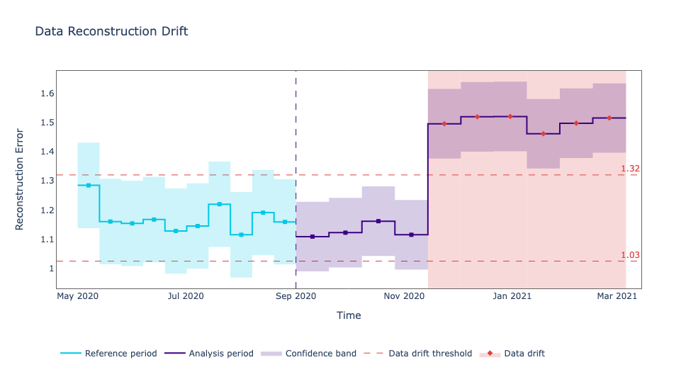
Looking at the plot above we see that indeed the reconstruction error went above the threshold after November 2020. Confirming our initial results. The post-production data is coming from a different distribution and this is affecting the model’s performance.

We as data scientists should care not only about getting nice train and test errors. But also about making sure that our production models are working as intended. Thankfully we have NannyML to babysit the models for us.

Conclusion#

By exploiting the capacities of NannyML you can monitor your machine learning models at all times, and be sure to detect any potential failure before it is too late.

This could not only save your company millions of dollars. But also give you hours of good night’s sleep knowing that nannyML is taking care of your machine learning system.

To learn more about how NannyML works and contribute to it check out github.com/nannyml